For a given voxel configuration, the diffusion signal  is simulated following the multi-tensor model as in [Tuch2004]:
where:
 is the coordinate vector in q-space, with
  and
and  .
. is the b-value corresponding to
  and diffusion time
  .
. is the number of fiber compartments, each one characterized by a self-diffusion tensor
  and a volume fraction
  , such that
  .
. is the signal amplitude without diffusion weigthing (
 ).
).Each diffusion tensor can be expressed as a rotated version of  as
as  . The tensor
  is a diagonal matrix whose elements are the diffusivities along the main axis of the
  fiber compartment (
 ) and in the plane perpendicular to it (
 ).
).  is the rotation matrix which rotates the z-axis in the direction of the fiber compartment.
Note
In this contest, we assume  without loss of generality.
Note
In this contest, the diffusivities are generated from the following ranges (see [Canales2009]) which are tipically found in the human brain: ![\lambda_1 \in [1,2] \: \times 10^{-3} \: \mathrm{mm}^2/\mathrm{s}](_images/math/5fcbc19d0c9fb4b04db6c052dbc5bd856e579198.png) and
and ![\lambda_2 = \lambda_3 \in [0.1,0.6] \: \times 10^{-3} \: \mathrm{mm}^2/\mathrm{s}](_images/math/0056b9f5eed8022ee3ffce9543bc9de932ccbf89.png) .
.
Note
In the code all fiber compartments are initially oriented along the z-axis. Thus, the diffusion profiles are specified in reverse order,  being the diffusivity along the main axis of the fiber compartment and
  in the plane perpendicular to it.
The MATLAB class in the MultiTensor.m file implements this model and can be used to simulate the signal at given q-space coordinates.
From the above definition, the Orientation Distribution Function (ODF) can be analytically computed as:
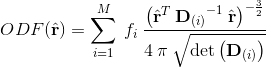
where  and
and  are, respectively, the inverse and the determinant of the diffusion tensor.
Rician noise is added to the signal in the following fashion:
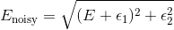
where 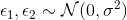 and
and  corresponds to a given signal-to-noise ratio (SNR).
For illustrative purposes, let’s create a voxel with a 90° fiber-crossing configuration:
% create the voxel configuration
VOXEL = MultiTensor();

% create two fiber compartments, with equal volume fraction and diffusivities
VOXEL.M = 2;
VOXEL.f = [ 0.5, 0.5 ];
VOXEL.lambda = [ 0.3 0.3 1.7 ; 0.3 0.3 1.7 ]' * 1e-3;

% create the rotation matrices to rotate the axis of the two fiber compartments
VOXEL.R(:,:,1) = VOXEL.ROTATION( 0, pi/2 );
VOXEL.R(:,:,2) = VOXEL.ROTATION( pi/2, pi/2 );
Now, let’s generate the signal of this configuration at b = 1000 mm2/s for the direction (1, 0, 0)T, with a noise level corresponding to an SNR = 50:
% specify the signal-to-noise ratio
SNR     = 50;
sigma   = 1 / SNR;

% specify the gradient direction and b-value
b       = 1000;
dir     = [ 1 0 0 ];

% acquire the signal at this q-space position and apply the noise
E       = VOXEL.E( b * dir );
E_noisy = VOXEL.addNoise( E, sigma );
To simplify the simulations, multiple q-space points can be probed for one voxel in one go by providing a text file (i.e. gradient_list.txt) with the list of coordinates (x, y, z, b):
SIGNAL = VOXEL.acquireWithScheme( 'gradient_list.txt', sigma );
The variable SIGNAL will contain then, for this voxel, one signal amplitude for each row of the file “gradient_list.txt”.
This section describes the general guidelines about the format of data and files exchanged throughout the contest. Should you have any more questions, please do not hesitate to contact us.
The gradient directions list must be a text file with:
Example:
 0.08796    -0.99612    0          1000
-0.11212    -0.98837    0.10271    1000
 0.017128   -0.98062   -0.19517    1500
 0.14077    -0.97287    0.18361    1500
-0.25782    -0.96512   -0.045605   2000
 0.24375    -0.95736   -0.15505    2000
    .           .          .         .
    .           .          .         .
    .           .          .         .
Each participant has the freedom to choose the acquisition scheme which suits best the needs of his own reconstruction method. He will send by e-mail to the organizers one “gradient_list.txt” text file with the coordinates of the q-space points to be sampled. Then, he will receive back from the organizers a MATLAB matrix (i.e. ”.mat” format) containing the diffusion signal simulated at each specified q-space position and for every voxel of the testing data phantom.
So, assuming the synthetic phantom has (nx, ny) voxels and the user needs to sample ns samples, then the resulting matrix containing the simulated signal will have a size equal to (nx, ny, ns).
Each participant should return to the organizers a file with the fibers configuration in each voxel of the testing data as estimated with their reconstruction technique. One separate file is requested for each synthetic phantom. Each such file should be a MATLAB structure (saved as a ”.mat” file) with two fields:
FIELD, which is a cell array containing the fiber configuration estimated with the participant’s proposed method:
- there must be one cell for each voxel of the corresponding synthetic phantom;
- each cell must be a “MultiTensor” object describing the fiber configuration in that voxel (i.e. number of fibers, orientations etc).
ODF, which is an array containing the corresponding estimated ODF:
- the ODF must be estimated for every direction specified in the ODF_XYZ.mat file (i.e. 724 directions on the unit sphere).
Assuming that the synthetic phantom has (nx, ny) voxels, then FIELD will have a size equal to (nx, ny), while ODF will be (nx, ny, 724).
References
| [Tuch2004] | Tuch. Q-ball imaging. Magnetic Resonance in Medicine, 52: 1358–1372 (2004) |
| [Canales2009] | Canales-Rodriguez et al. Mathematical description of q-space in spherical coordinates: exact q-ball imaging. Magnetic Resonance in Medicine, 61: 1350–1367 (2009) |