The Isolated Voxels synthetic phantom (Training_IV.mat file) consists in an array of voxels each containing a different fiber configuration, as previously described. In particular:
The Structured Field synthetic phantom (Training_SF.mat file) consists in a 2D slice made up of 4 different fiber bundles as shown in the following figure. It is stored as a 10 x 10 cell array, each cell containing an object of the class MultiTensor. Each of these 4 fiber bundles was generated with specific diffusivities, in the given ranges as before, and are coherent along the bundle itself. However, different bundles might have different diffusion profiles.
Note
Even though the phantom consists in a 2D slice, the fibers can be oriented in every direction in the 3D space. Please have a look, for instance, at the blue bundle in the upper corner which crosses the plane perpendicularly.
Important
Following some valuable comments received from participants requesting for more testing data, we decided to release an additional synthetic phantom made up of several 3D slices.
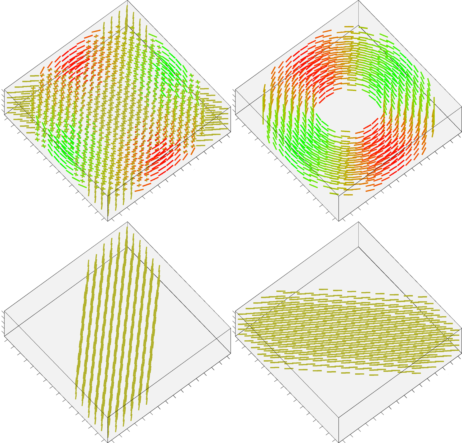
The additional Structured Field synthetic phantom (Training_3D_SF.mat file) consists in a 3D volume made up of 5 slices, and contains 3 different fiber bundles as shown in figure 2. It is stored as a 16 x 16 x 5 cell array, each cell containing an object of the class MultiTensor as before. The data has been generated as the previous datasets, with combinations of straight and bending trajectories. The code previously provided can be actually used in the same way: simply iterate over x, y and z instead of x and y only.

FIGURE 2. A screenshot of the additional Structured Field phantom. This synthetic dataset is made up now by 5 different slices.
The training data can be downloaded here.
Just uncompress the ZIP archive and you’ll find the three synthetic phantoms “Training_IV.mat”, “Training_SF.mat” and the new “Training_3D_SF.mat” in the folder called “Phantoms”. Each file contains a cell array named “FIELD”.
The following code snippet shows an “template” script for processing the data:
%% (STEP 1) Create the SAMPLING SCHEME
%  ===================================

%
% write here your own code to create the text file (i.e. "gradient_list.txt")
% containing the SAMPLING SCHEME needed by your recostruction method
%


%% (STEP 2) Simulate the SIGNAL for each voxel, phantom and SNR
%  ============================================================
SNRs          = [ 10 20 30 ];
PHANTOM_names = { 'Training_IV', 'Training_SF', 'Training_3D_SF' }; % in the folder "Phantoms"

% load the SAMPLING SCHEME
XYZB = dlmread( 'gradient_list.txt', ' ' );
nSAMPLES = size( XYZB, 1 );

for PHANTOM_name = PHANTOM_names
    load( fullfile('Phantoms',PHANTOM_name{1}) ) % load the variable "FIELD"
    [n1,n2,n3] = size( FIELD );

    for SNR = SNRs
        sigma = 1 / SNR;
        E = zeros( [n1 n2 n3 nSAMPLES], 'single' );
        for x = 1:n1
        for y = 1:n2
        for z = 1:n3
            VOXEL = FIELD{x,y,z};
            E(x,y,z,:) = VOXEL.acquireWithScheme( XYZB, sigma );
        end
        end
        end
        save( sprintf('%s__SNR=%02d__SIGNAL.mat', PHANTOM_name{1}, SNR), 'E' )
    end
end

%
% NB: in the case of the "testing data", simply send the file "gradient_list.txt"
% to the organizers, and you'll receive back the SIGNAL simulated as in the code
% snipped above (this is the code we actually use)
%


%% (STEP 3) Reconstruct each voxel with your own method
%  ====================================================
for PHANTOM_name = PHANTOM_names
for SNR = SNRs

    % load the SIGNAL simulated with this SNR
    load( sprintf('%s__SNR=%02d__SIGNAL.mat', PHANTOM_name{1}, SNR) )
    [n1,n2,n3,~] = size( E );

    % reconstruction of the configuration in each voxel
    myESTIMATION = [];
    myESTIMATION.FIELD = cell(  n1, n2, n3 );
    myESTIMATION.ODF   = zeros( n1, n2, n3, 724 );

    %
    % write here your own code to apply your RECONSTRUCTION METHOD
    % to this data and store the results in the structure "myESTIMATION"
    % (what follows is just an illustrative example)
    %

    for x = 1:n1
    for y = 1:n2
    for z = 1:n3
        % create the MultiTensor object
        myESTIMATION.FIELD{x,y,z} = MultiTensor();

        % number of fiber compartments in this voxel
        myESTIMATION.FIELD{x,y,z}.M = ?????;

        % relative volume fractions and diffusivities for each estimated fiber compartment
        myESTIMATION.FIELD{x,y,z}.f = [ ??, ??, ... ];
        myESTIMATION.FIELD{x,y,z}.lambda = [ ?? ?? ?? ; ?? ?? ??; ... ]' * 1e-3;

        % orientation of each fiber compartment
        myESTIMATION.FIELD{x,y,z}.R = zeros( 3, 3, myESTIMATION.FIELD{x,y,z}.M );
        for d = 1:myESTIMATION.FIELD{x,y,z}.M
            myESTIMATION.FIELD{x,y,z}.R(:,:,d) = myESTIMATION.FIELD{x,y,z}.ROTATION( ??, ?? );
        end

        % estimate the ODF in this voxel
        % (please use the directions in the file ODF_XYZ.mat)
        myESTIMATION.ODF(x,y,z,:) = [ ????? ];
    end
    end
    end

    % save the results
    save( sprintf('%s__SNR=%02d__myESTIMATION.mat', PHANTOM_name{1}, SNR), 'myESTIMATION' );
end
end

%
% NB: in the case of the "testing data", simply send these files
% to the organizers for the evaluation of the reconstructions
%
Both the Isolated Voxels and the Structured Field synthetic phantoms were generated with the same code and conventions as for the Training data. The dimensions of the two phantoms have been increased as requested by some groups. The former phantom now consist of a cell array 10 times bigger than before, while the latter is a 3D volume with 16 x 16 x 5 voxels (as was the case for the latest training data). Of course, the configuration in each voxel has changed and is unknown to the participants. The ground-truth will be revealed after the evaluations of the reconstructions.
Note
The testing data must be unknown to the contestants, so it is not possible to “download” it! As already stated, to simulate the signal to be used for testing your method simply send the file “gradient_list.txt” to the organizers, and you’ll receive back the SIGNAL simulated as in the code snipped above.
The signal will be simulated with different levels of noise (SNR = 5, 10, 15, 20, 25, 30, 35, 40). However, only the reconstructions corresponding to SNR = 10, 20, 30 will be considered for the final ranking. The remaining data will be used only for illustrative purposes, in order to provide a more comprehensive comparison to have more fruitful discuss during the final workshop.
The gound-truth for the testing data can be downloaded here.